What Is Personalized Regression? Patient-Specific Genetic Effects
Standard regression gives everyone the same coefficients. Personalized regression gives each person their own, even though each person is only one row of data. Here is how that can work, with a small example you can check by hand.
By Jiahui Zhang, Haohan Wang, and others · · About our npj Dementia 2026 paper
What is personalized regression? It is a way to fit a separate set of coefficients for every sample, so that a genetic variant can matter for one patient and not for another. The difficulty is that one patient is a single row of data, so the method has to borrow from other patients without erasing what makes each one different. This post explains heteroscedastic personalized regression (Het-PR), from Stratifying Alzheimer's disease by patient-specific genetic signatures reveals cognition-linked and cross-disease heterogeneity, by Jiahui Zhang, Ziyu Yu, Xingcai Zhang and Haohan Wang (University of Illinois Urbana-Champaign and Stanford University School of Medicine, npj Dementia, 2026). Het-PR fits one weighted regression per person, and in that study it produced a profile over 1,684 SNPs for each of 251 Alzheimer's patients.
Key findings
- Heteroscedastic personalized regression (Het-PR; Zhang, Yu, Zhang and Wang, npj Dementia 2026, University of Illinois Urbana-Champaign) estimates one person's coefficients by fitting all samples and treating the difference between that person and everyone else as extra noise, which grows with distance on background covariates, so all 815 people in its Alzheimer's analysis inform each person's estimate.
- In the Alzheimer's Disease Neuroimaging Initiative (ADNI), Het-PR ran on 815 people (251 with Alzheimer's, 564 controls), with 1,684 exonic SNPs as features and 72,842 background SNPs defining similarity, and needed no tuned similarity scale because that scale was fixed in advance.
- In the npj Dementia paper's structured-subgroup simulations, where the similarity matrix came from the true groups, Het-PR found truly influential SNPs at AUROC 0.82–0.94 while baselines rarely exceeded 0.65, and clustering its scores recovered hidden subgroups with 90–100% accuracy.
- The gain shrinks when the similarity information is weak: in the paper's sensitivity analysis on ADNI-derived genotypes, Het-PR's AUROC was 0.945 with oracle covariates and 0.914 with random ones, against 0.901 for a population model, and with no subgroups at all both scored 1.000.
Note for patients and families: this post is about a statistical research method. "Patient-specific" here means a score computed for each research participant, not a test that a doctor can order, and it says nothing about what any individual should do. If you have questions about genetic risk or memory changes, a neurologist or genetic counselor is the right person to ask.
Why isn't one regression enough for everyone?
Most genetic association studies estimate one effect per variant for the whole cohort. As the paper puts it, these traditional models treat all individuals as sharing a common genetic architecture. That is a reasonable start, and it is how many Alzheimer's risk loci were found. But if a variant pushes the outcome up in some people and has no effect or the opposite effect in others, the single average describes neither group.
For the clinical side of this problem, see our earlier posts on the same paper: Are there genetic subtypes of Alzheimer's disease? covers the subgroups and memory differences, and Is there a genetic link between Alzheimer's and epilepsy? covers the cross-disease result. This post is about the method underneath them.
Key terms
- Personalized regression
- A regression that gives each sample its own coefficients and borrows from other samples to make them estimable.
- Sample-specific model
- The general name in machine learning for a model with parameters that belong to one sample rather than to a whole population.
- Heteroscedastic noise
- Noise whose variance differs between observations, so some data points are trusted less than others.
- Heteroscedastic personalized regression (Het-PR)
- A personalized regression that estimates each target person's coefficients from all samples by giving more distant samples larger noise variance.
- Background covariates (the matrix C)
- The variables used to decide who counts as similar to whom; in the ADNI analysis, 72,842 SNPs outside the feature set.
- Linear mixed model (LMM)
- A regression with fixed effects plus random effects, widely used in genome-wide association studies.
- AUROC
- A score from 0.5 (chance) to 1.0 (perfect) for how well a method ranks true signals above false ones.
Why can't you just fit a regression for each person?
Ordinary linear regression assumes one coefficient vector β for all n samples:
Personalized regression replaces it with a vector βi for each sample i:
Now there are n times as many unknowns, and, as the paper notes, each βi is supported by only a single sample. One row cannot determine many coefficients, so every personalized method needs an extra assumption. The classic one, from Lengerich, Aragam and Xing, is that samples with similar covariates should have similar coefficients.
How does heteroscedastic personalized regression work?
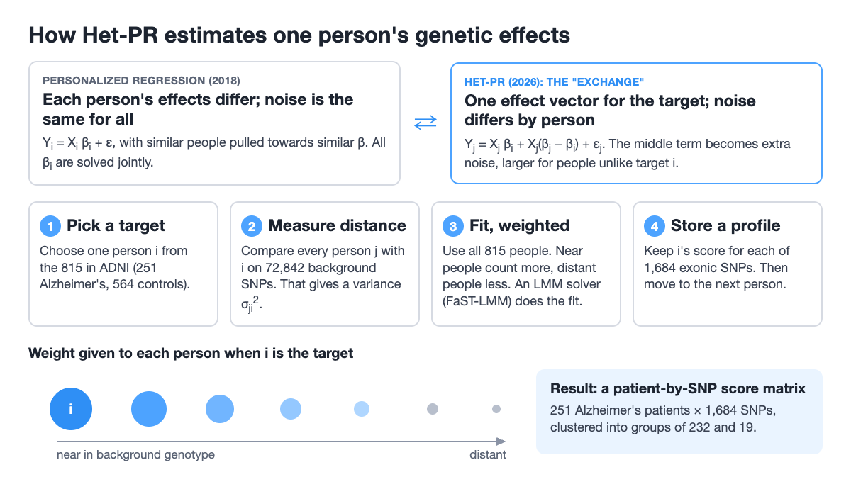
Het-PR's idea is to move the variation from the coefficients into the noise. The paper calls this an "exchange": instead of a model with a different coefficient vector per person and the same noise for everyone, it uses a model that is homogeneous in the coefficients, with error variance that differs across samples.
Fix a target person i. For anyone else, j, add and subtract the same term:
This is plain algebra, and it says that person j's outcome can be written with person i's coefficients plus a discrepancy. Het-PR then treats the discrepancy as a zero-mean Gaussian term with variance σji2. That variance cannot be computed from the unknown coefficients, so it is tied to something observable, the distance between the two people on the background covariates:
Every person now contributes to the estimate of βi, but someone far from the target carries a large variance and so a small effective weight. The target's own row has σii2 = 0. Repeat for each target, and you have a coefficient vector per person.
The paper is explicit that this is a statistical working design. It does not claim that differences between Alzheimer's patients are unstructured random noise; the Gaussian term is a variance-weighting approximation that makes each person's estimate feasible.
Can you show personalized regression with a worked example?
Yes. The numbers below are made up by us to show the mechanics; they are not from the paper. Six people have a dosage x of one SNP and an outcome y. The true effect is +1 for P1–P3 and −1 for P4–P6, and nobody has told the model which is which. With no intercept and a noise variance σε2 = 0.1, take P1 as the target. Each person's variance is σj12x2 + 0.1, and each weight is one over that variance.
| Person | SNP dosage x | Outcome y | Background distance to P1 (σj12) | Variance | Weight | Share of total weight |
|---|---|---|---|---|---|---|
| P1 (target) | 2 | 2.1 | 0 | 0.10 | 10.00 | 39.5% |
| P2 | 1 | 0.9 | 0.02 | 0.12 | 8.33 | 33.0% |
| P3 | 2 | 1.9 | 0.02 | 0.18 | 5.56 | 22.0% |
| P4 | 1 | −1.1 | 1 | 1.10 | 0.91 | 3.6% |
| P5 | 2 | −1.9 | 1 | 4.10 | 0.24 | 1.0% |
| P6 | 2 | −2.1 | 1 | 4.10 | 0.24 | 1.0% |
The weighted least-squares slope is Σwxy / Σwx2 = 0.92 for P1. One ordinary regression on all six gives Σxy / Σx2 = −0.2 / 18 = −0.01, which says that the SNP does nothing. Swap the target to P5, with the distances reversed, and the same calculation gives −0.92. Nobody was dropped from either fit; the weights did the work.
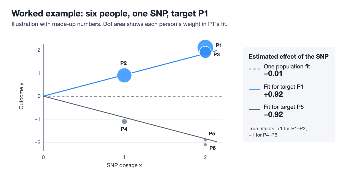
Two simplifications to keep in mind. The real model has many features, and it runs through a mixed-model solver instead of this one-line formula. And here we chose distances that happen to line up with the true groups; in real data the distances come from C, which may line up much less well. The simulation results below show what that costs.
How is Het-PR applied to real genetic data?
The ADNI analysis is a good example of the choices a user has to make.
- Outcome. Alzheimer's versus cognitively normal diagnosis at the baseline visit, for 815 people (251 Alzheimer's, 564 controls). Demographic covariates were regressed out first, and the standardized residuals were used as the outcome.
- Features X. 1,684 exonic SNPs in Alzheimer's-related genes.
- Background C. The remaining 72,842 SNPs, used only to measure who is similar to whom.
- Similarity scale. γ was not tuned by cross-validation or grid search. The squared distance was divided by the number of background SNPs m, which is the same as fixing γ = 1/√m.
- Fit. Equation 12 of the paper has the same Gaussian form as a linear mixed model with a sample-specific variance, so each target's fit runs through the FaST-LMM algorithm. The paper reports that overall cost scales linearly with n because the fit is repeated once per sample.
- Output. For each person and SNP, a working-likelihood score: the paper's term is an "individualized association score", the local evidence that the SNP helps separate Alzheimer's from controls for that person under the model.
- Use. Scores for the 251 patients were transformed to −log10, then clustered hierarchically, which gave groups of 232 and 19 patients. The split was unchanged in 500 runs that each used 80% of the patients.
The same recipe can in principle personalize other base models. The paper writes a general form for any regression function f(X; Θ), where the variance term uses the model's Jacobian with respect to its parameters, so nonlinear models fit the framework on paper. The ADNI analysis used the linear version, and the two base models in the simulations were a linear mixed model variant and standard linear regression.
The code is at github.com/zjh688/Het-PR and runs on your
own prepared data with python runHetPr.py fit -t csv -n toyData. The repository holds the
model and data pipeline; scripts for reproducing the paper's experiments are available from the
authors. ADNI data require an application and a data use agreement.
Does personalized regression recover true effects in simulations?
Yes in the settings tested, though by how much depends a lot on the setting. The main benchmark split samples into cohorts with different sparse effect vectors, across 27 configurations of sample size, feature count, sparsity and number of cohorts, with five runs each. C was the true cohort information, so similarity was correctly specified by construction.
| Structured-subgroup benchmark (oracle C) | Het-PR | Alternatives |
|---|---|---|
| AUROC for finding truly influential SNPs | typically 0.82–0.94 | baselines rarely above 0.65 |
| Recovering latent subgroups by clustering scores | 90–100% accuracy; AUROC near 0.95 in most settings | subgroup AUROC often close to 0.5 |
From the Simulation results section of the paper. The baselines were a distance-matching personalized regression, penalized angular regression, a clustering regression and a population regression. In the supplement, Het-PR scored higher than the others in nearly all cases, with one stated exception: a clustering regression that was told the true clusters.
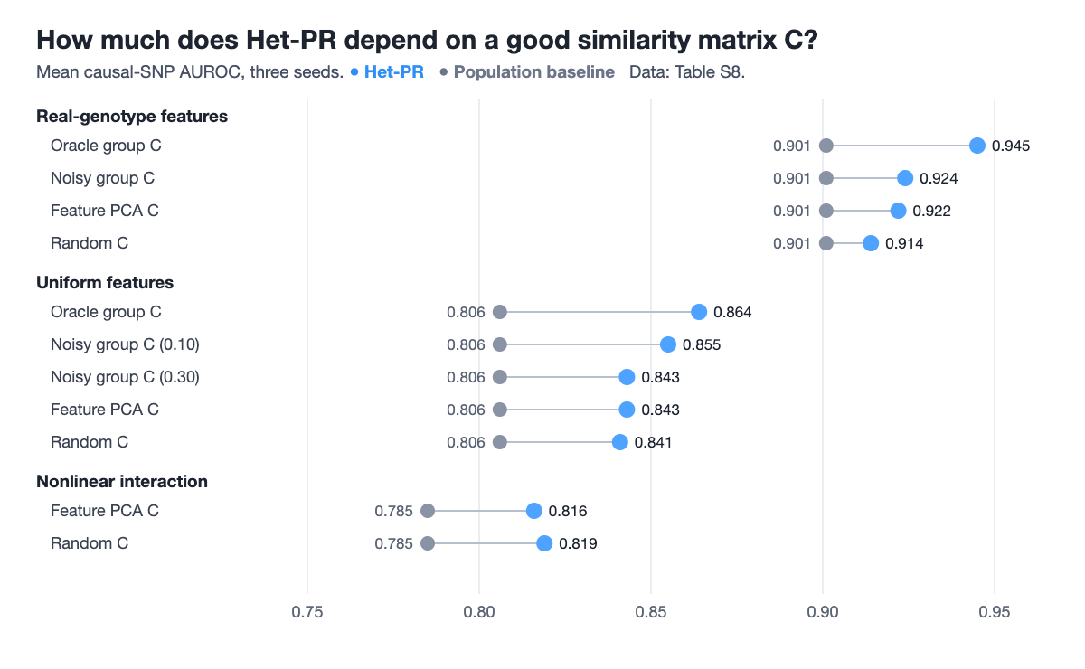
An oracle C is a generous test, and the authors ran a sensitivity analysis to check how much it helped. There, C was replaced by noisy group labels, principal components of the features, or random numbers:
| Scenario | Features | C | Het-PR AUROC | Population AUROC |
|---|---|---|---|---|
| Structured subgroups | Real genotype | Oracle group | 0.945 | 0.901 |
| Structured subgroups | Real genotype | Noisy group (0.30) | 0.924 | 0.901 |
| Structured subgroups | Real genotype | Feature PCA | 0.922 | 0.901 |
| Structured subgroups | Real genotype | Random | 0.914 | 0.901 |
| Structured subgroups | Uniform | Oracle group | 0.864 | 0.806 |
| Structured subgroups | Uniform | Noisy group (0.10) | 0.855 | 0.806 |
| Structured subgroups | Uniform | Noisy group (0.30) | 0.843 | 0.806 |
| Structured subgroups | Uniform | Feature PCA | 0.843 | 0.806 |
| Structured subgroups | Uniform | Random | 0.841 | 0.806 |
| Nonlinear interaction | Uniform | Feature PCA | 0.816 | 0.785 |
| Nonlinear interaction | Uniform | Random | 0.819 | 0.785 |
| No subgroups | Uniform | Feature PCA | 1.000 | 1.000 |
| No subgroups | Uniform | Random | 1.000 | 1.000 |
From Table S8 of the paper's supplement: mean sample-level causal-SNP AUROC across three seeds.
Three readings. Better similarity information helps, since oracle C is the top score in both feature settings. Het-PR did not fall below the population model when C was noisy or even random, and when there were no subgroups at all it simply matched it, so personalizing did no harm here. And the margins in this table are much smaller than the 0.82–0.94 versus 0.65 contrast above. The population baseline scores far higher here than the baselines in the main benchmark, so the two sets of numbers appear to come from different simulation setups and should not be read side by side. For planning a real analysis, we think this table is the more cautious guide.
There is also a check on real data. In a negative control, the Alzheimer's and control labels were shuffled and Het-PR was refitted 50 times. The share of patient-SNP scores at or below 0.05 was 5.66% with the real labels, against a shuffled median of 4.13% and a range of 2.49–10.83%. So the count of scores passing the threshold is not evidence of signal, and the authors do not use it as such: it is a calibration reference showing that the scores behave close to their null at that level.
How does Het-PR compare with mixed models and other sample-specific methods?
Het-PR sits in a long line of models whose parameters vary across samples:
| Approach | What varies | How samples share information |
|---|---|---|
| Population regression | Nothing: one β for all | All samples count equally |
| Mixture of regressions | A few group-level models | Samples in a component share one model |
| Varying-coefficient model | β as a smooth function of covariates | Through that function |
| Contextualized model | β from a learned context encoder | A deep network maps context to parameters |
| Personalized regression (distance matching) | A βi per sample | Joint fit; coefficient distances match covariate distances |
| Low-rank personalized regression | A βi per sample, in a shared low-rank dictionary | Shared dictionary plus distance matching |
| Bayesian hierarchical model | Subject effects drawn from a population prior | Shrinkage towards the population |
| Het-PR | A βi per target person | Separate fit per target; variance grows with distance |
- Personalized regression. Personalized regression enables sample-specific pan-cancer analysis (Benjamin Lengerich, Bryon Aragam and Eric Xing, Carnegie Mellon University, Bioinformatics, 2018) is the work Het-PR builds on. It starts from a population lasso fit and uses a distance-matching regularizer, so that distances between coefficient vectors track distances between covariates, on TCGA data with 9,663 RNA-seq profiles (8,944 cases and 719 matched controls). Its joint formulation states the problem directly; Het-PR is a different route to the same target.
- Low-rank personalized regression. Learning Sample-Specific Models with Low-Rank Personalized Regression (Lengerich, Aragam and Xing, NeurIPS 2019) factorizes the coefficient matrix through a shared dictionary, cutting the parameter count from about np to q(n + p), and fits over 10,000 samples and thousands of predictors in under an hour on a laptop. On a mass-spectrometry cancer task it reports test AUROC 0.923, against 0.794 for a population model and 0.876 for a mixture of regressions. Where it estimates all samples jointly in a compressed space, Het-PR fits each target separately.
- Varying-coefficient models. Varying-Coefficient Models (Trevor Hastie and Robert Tibshirani, Journal of the Royal Statistical Society: Series B, 1993) let coefficients vary as smooth functions of other variables. This is the classic statistical ancestor, and a good choice when a meaningful covariate such as age drives the change.
- Contextualized models. Contextualized Machine Learning (Lengerich, Ellington, Rubbi, Kellis and Xing, arXiv, 2023) applies deep learning to the relationship between context and context-specific parametric models, with an accompanying PyTorch package. Evolution of Personalized Models by Caleb Ellington is a clear map of this whole family.
- Linear mixed models. FaST linear mixed models for genome-wide association studies (Lippert, Listgarten, Liu, Kadie, Davidson and Heckerman, Nature Methods, 2011) is an algorithm that scales linearly with cohort size in run time and memory, and its authors report analyzing 120,000 individuals in a few hours. Het-PR uses this machinery for computation only. Its likelihood has the same form as a mixed model, but the variance comes from the working discrepancy term and the C-based weighting, not from population-level random effects, so the paper does not read it as a conventional random effect.
- Bayesian hierarchical models. As the paper describes them, these place a population distribution or prior over subject-level coefficients and return posterior or shrinkage estimates. Het-PR builds a working likelihood for each target instead, so its output is a score profile, not a posterior distribution. If you need calibrated uncertainty about a person's effect, a hierarchical model is the more direct tool.
When should you use personalized regression?
Our reading of the results above, as practical guidance:
- It suits exploration. Use it when you suspect that effects differ between people, you have no labels for the groups, and you want profiles to cluster or inspect.
- You need a defensible C. The method is only as personal as its similarity measure. Choose C before looking at the results, and keep it separate from the features, as the ADNI analysis did.
- It adds little if effects are shared. In the no-subgroup simulation, Het-PR matched the population model. A population analysis remains the simpler first step.
- Validate downstream. Treat the scores as a way to generate structure, then test that structure against information the model never saw, as the paper did with memory measures and trait-associated variants.
What this does not show
- Scores are not measured effects. Het-PR outputs are model-derived association scores, conditional on the working likelihood and on C. A per-patient score is not a validated finding that a SNP acts in that person, and it is not a causal estimate.
- No individual-level ground truth. In real data nobody knows a patient's true coefficients. The evidence for accuracy comes from simulations, where the truth is known by construction.
- Scores near their null at p ≤ 0.05. With shuffled labels, the share of passing scores (median 4.13%) was close to the observed 5.66%. Downstream structure, not the raw count of passing scores, is what the paper relies on.
- The gain depends on C. With random C on ADNI-derived genotypes, the margin over a population model was 0.914 versus 0.901.
- A working assumption. Treating differences between people as Gaussian noise is an approximation. The authors note that real differences may be structured, and they suggest explicit mixture or subgroup-aware extensions as future work.
- Limited covariates. In ADNI, demographics entered only through outcome residualization, and C held SNPs alone. Comorbidities, medication and environment were not modeled.
- One real cohort. The Alzheimer's application uses ADNI only, with a 19-patient subgroup and no independent replication.
- The nonlinear form is largely untested. The general formula covers nonlinear models, but the experiments used linear base models; nonlinear effects were tested only as data that a linear-base model had to cope with.
- Not a clinical tool. This is a research method. It does not give a diagnosis, a risk estimate or a treatment recommendation.
Frequently asked questions
What is personalized regression?
Personalized regression is a family of methods that gives every sample its own regression coefficients instead of one set shared by everyone. Because one person's data cannot fix many coefficients alone, each method adds a rule for borrowing from other samples, usually that similar samples should have similar coefficients. The idea was introduced for genomics by Lengerich, Aragam and Xing (Bioinformatics, 2018).
How do you estimate patient-specific genetic effects?
You need a way to borrow strength across patients, since each patient supplies only one row of data. Heteroscedastic personalized regression (Het-PR, npj Dementia 2026) does this by fitting one weighted regression per target patient on the whole cohort, giving less weight to people whose background genotype is far from the target. The output is a model-derived association score per patient and SNP, not a measured causal effect.
How is personalized regression different from a linear mixed model?
A linear mixed model in genetics estimates population-level effects and uses random effects for population-level structure. Het-PR estimates coefficients for one target person at a time. Its likelihood has the same algebraic form as a mixed model with a sample-specific variance, which lets it reuse fast solvers such as FaST-LMM, but its variance term is a weighting device, not a random effect.
Is personalized regression the same as a polygenic risk score?
No. A polygenic risk score estimates a person's genetic liability to a trait from their genotype and data from a genome-wide association study, so it gives one number per person for that trait. Personalized regression instead estimates a separate profile of associations per person, one value for each variant, and it is a research method rather than a risk test.
Citation
@article{zhang2026stratifying,
  title   = {Stratifying Alzheimer's disease by patient-specific genetic signatures reveals cognition-linked and cross-disease heterogeneity},
  author  = {Zhang, Jiahui and Yu, Ziyu and Zhang, Xingcai and Wang, Haohan},
  journal = {npj Dementia},
  volume  = {2},
  pages   = {90},
  year    = {2026},
  doi     = {10.1038/s44400-026-00124-5}
}
References
- Zhang J, Yu Z, Zhang X, Wang H. Stratifying Alzheimer's disease by patient-specific genetic signatures reveals cognition-linked and cross-disease heterogeneity. npj Dementia 2, 90 (2026). doi:10.1038/s44400-026-00124-5
- Chen Z, Wang H. Heteroscedastic personalized regression unveils genetic basis of Alzheimer's disease stratified by cognitive level. bioRxiv (2023). doi:10.1101/2023.09.12.557499
- Lengerich BJ, Aragam B, Xing EP. Personalized regression enables sample-specific pan-cancer analysis. Bioinformatics 34(13), i178–i186 (2018). doi:10.1093/bioinformatics/bty250
- Lengerich B, Aragam B, Xing EP. Learning sample-specific models with low-rank personalized regression. Advances in Neural Information Processing Systems (NeurIPS 2019). arXiv:1910.06939
- Hastie T, Tibshirani R. Varying-coefficient models. Journal of the Royal Statistical Society: Series B 55(4), 757–779 (1993). doi:10.1111/j.2517-6161.1993.tb01939.x
- Lengerich B, Ellington CN, Rubbi A, Kellis M, Xing EP. Contextualized machine learning. arXiv (2023). arXiv:2310.11340
- Lippert C, Listgarten J, Liu Y, Kadie CM, Davidson RI, Heckerman D. FaST linear mixed models for genome-wide association studies. Nature Methods 8, 833–835 (2011). doi:10.1038/nmeth.1681
- Choi SW, Mak TSH, O'Reilly PF. Tutorial: a guide to performing polygenic risk score analyses. Nature Protocols 15, 2759–2772 (2020). doi:10.1038/s41596-020-0353-1
Related from our lab
- Are there genetic subtypes of Alzheimer's disease? The Het-PR subgroups and their memory differences
- Is there a genetic link between Alzheimer's and epilepsy? The cross-disease result from the same paper
- Why Alzheimer's patients with the same diagnosis differ: an essay by Haohan Wang
- Gene regulation and disease genetics, including Alzheimer's heterogeneity: research overview by Haohan Wang
- Can AI agents analyze gene expression data like experts? GenoMAS, GenoTEX and SCTA
- This paper and our other peer-reviewed work on Alzheimer's disease and computational genomics